[Home]
[Table of Contents] [Next Section]
SWMU Demo Dud Area (DD) Area Closure Report
Section 2 - Closure Activities
The recommendations of the 2002 RFI Report were to evaluate the extent of contamination with surface and subsurface samples. Following contamination evaluation, the area was to be excavated to remove all waste and waste residue present at the site.
2.1 - Excavation and Disposal
Excavation activities commenced on November 20, 2003 to remove any contaminated soils remaining at the site after the initial excavation/sifting activities completed in 1997. Further excavation and scraping of hot spots occurred during January, February, April, and May 2004 to remove remnant contamination. Approximately 1,630 cubic yards of soil were excavated. These soils were stockpiled, characterized, and disposed with the 600 CY generated during the 1997 excavation (2,230 CY total disposed).
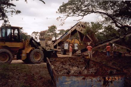
Excavated material was stockpiled onsite so that the material could be characterized for disposal. Disposal of the waste was conducted under waste profile CG‑26901, C‑6. Waste manifests are provided in Appendix A. Toxicity characteristic leaching procedure (TCLP) results from the stockpiled waste indicated the material met Class 2 concentrations, so the waste was disposed at Covel Gardens Landfill, San Antonio, TX. The following photographs show excavation activities at the site.
Sifting removed soils - May 1997
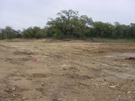
Excavation area at site - January 2004
Confirmation sampling was performed to verify that RRS1 criteria had been met. After the waste and waste residue were excavated, samples were collected on the sidewalls and the bottom of the excavated area. If any samples came back above RRS1 limits, the area that the sample was collected from was further excavated and resampled to verify that all waste and waste residue was removed. Thirty‑one sidewall samples and five bottom samples were collected. Sample locations are displayed in Figure DD‑7.
2.2.1 Confirmation Sampling Methodology
Each closure sample was analyzed for the site contaminants of concern (COCs) determined through previous investigations and included toluene (SW8260B), SVOCs (SW8270C), copper and zinc (SW6010B), lead (SW7421), and mercury (SW7471A).
2.2.2 Confirmation Sampling Results
Samples were analyzed for toluene, copper, zinc, lead, mercury and SVOCs. The sampling suite was determined by the analytes that exceeded RRS1 criteria in the RFI sampling results. The sample results can be found in Table DD‑3.
After samples were collected and results were received, overexcavation was conducted at sampling locations with RRS1 exceedances and samples were collected from the overexcavated area. These samples were analyzed for only those analytes that exceeded RRS1 in the original sample. Some locations needed to be overexcavated more than one time before all waste residue was removed and the sample results achieved RRS1. The sample results are presented in Table DD‑3.
Analytical results for overexcavation samples were reported below the RRS1 limits; however, lead, mercury, and di‑n‑butylphthalate still had RRS1 exceedances after overexcavation activities were complete.
To further excavate the remaining exceedances for possible closure, 30 TAC §334.443(d)(2) allows use of statistical comparison using the 95 percent confidence limit of the mean concentration of the contaminant as a representative value for the site. If all the sample results across the site are used to calculate an upper confidence limit (UCL), and the UCL is less than the established background level, then the site can be closed under RRS1.
To calculate the UCL, the data must be normally or log‑normally distributed. To test the distribution of the data, the Shapiro‑Wilk test (W) of normality is used (if sample sizes are less than or equal to 50). The Shapiro‑Wilk test is included in the EPA software, ProUCL, used for the UCL calculations (EPA 2003; also located at: http://www.epa.gov). If the distribution is normal, the UCLs are calculated on the raw data. If the distribution is not normal, then the data are log transformed, and the Shapiro‑Wilk test of normality is applied to the transformed data. If the data are log‑normally distributed, the UCLs are calculated based on the transformed data. If the test statistic W exceeds the critical value, then that distribution is considered normal or log‑normal, according to the distribution of the data. The appropriate UCL calculation for log‑normally distributed data is based on the standard deviation (σ) of the data. If σ <0.5, or 0.5 ≤ σ <1.0, the H‑UCL is recommended. If 1.0 ≤ σ <1.5, then the 95% Chebyshev UCL is recommended, to account for the skewness of the data.
A total of 38 samples collected for closure were used for the statistical analyses, but not all samples were used for all analytes. If a sample had a duplicate sample collected, the higher result for the two samples was used for statistical evaluation. For each analyte, the distribution of the data was tested for normality as described above. Statistical evaluations can be found in Appendix B.
Data flags were treated in the following way for data analysis. If the data were flagged with an F, J, or B flag, the concentrations were retained in the data set. If the data were flagged with a U flag, the concentration was entered as one‑half the value of the sample quantitation limit (SQL).
Lead exceeded background levels at only one location, DD‑SW21, with a concentration of 206.13 mg/kg; the CSSA background concentration is 84.5 mg/kg. For this data, there were a total of 14 samples used in the UCL calculation, and the critical Shapiro‑Wilk test (W) of normality was 0.874. The data are log‑normally distributed (W = 0.957). The σ = 1.13 for the transformed data, and the calculated 95% Chebyshev UCL is 74.54 mg/kg lead, which is less than the CSSA background concentration. Since the calculated UCL for lead does not exceed the CSSA background level and meets the requirements for RRS1 closure.
Mercury exceeded CSSA background levels of 0.77 mg/kg at one location, DD‑SW02, with a concentration of 0.96 mg/kg. There were a total of 16 samples used in the UCL calculation, and the critical W = 0.874. The data are log‑normally distributed (W = 0.916). The σ = 1.25 for the transformed data, and the calculated Chebyshev UCL is 0.61 mg/kg, which is less than the CSSA background concentration. Because the calculated UCL for mercury does not exceed the CSSA background level and meets the requirements for RRS1 closure.
Di‑n‑butylphthalate exceeded the RL of 0.77 mg/kg at one location, DD‑BOT01, with a concentration of 0.86 mg/kg. There were a total of 14 samples used for the UCL calculation, and the critical W = 0.874. The data are normally distributed (W = 0.976). The calculated UCL is 0.57 mg/kg, which does not exceed the RL. Because the calculated UCL for di‑n‑butylphthalate does not exceed the RL concentration and meets the requirements for RRS1 closure.