Three-Tiered LTMO Section 6 - Spatial Statistical Evaluation

Spatial statistical techniques also can be applied to the design and evaluation of groundwater monitoring programs to assess the quality of information generated during monitoring, and to evaluate monitoring networks. Geostatistics, or the Theory of Regionalized Variables (Clark, 1987; Rock, 1988; American Society of Civil Engineers Task Committee on Geostatistical Techniques in Hydrology, 1990a and 1990b), is concerned with variables having values dependent on location, and which are continuous in space, but which vary in a manner too complex for simple mathematical description. Geostatistics is based on the premise that the differences in values of a spatial variable depend only on the distances between sampling locations, and the relative orientations of sampling locations--that is, the values of a variable (e.g., chemical concentration) measured at two locations that are spatially "close together" will be more similar than values of that variable measured at two locations that are "far apart".

Ideally, application of geostatistical methods to the results of the groundwater monitoring program at CSSA could be used to estimate COC concentrations at every point within the dissolved contaminant plume, and also could be used to generate estimates of the �error,� or uncertainty, associated with each estimated concentration value. Thus, the monitoring program could be optimized by using available information to identify those areas having the greatest uncertainty associated with the estimated plume extent and configuration. Conversely, sampling points could be successively eliminated from simulations, and the resulting uncertainty examined, to evaluate whether significant loss of information (represented by increasing error or uncertainty in estimated chemical concentrations) occurs as the number of sampling locations is reduced. Repeated application of geostatistical estimating techniques, using tentatively identified sampling locations, could then be used to generate a sampling program that would provide an acceptable level of uncertainty regarding the distribution of COCs with the minimum possible number of samples collected. Furthermore, application of geostatistical methods can provide unbiased representations of the distribution of COCs at different locations in the subsurface, enabling the extent of COCs to be evaluated more precisely.

Fundamental to geostatistics is the concept of semivariance [g(h)], which is a measure of the spatial dependence between sample variables (e.g., chemical concentrations) in a specified direction. Semivariance is defined for a constant spacing between samples (h) by:

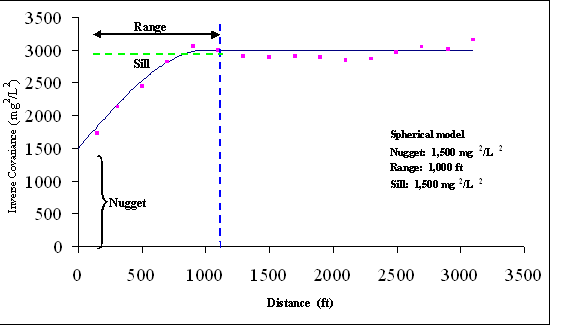
Semivariograms (plots of g(h) versus h) are a means of depicting graphically the range of distances over which, and the degree to which, sample values at a given point are related to sample values at adjacent, or nearby, points, and conversely, indicate how close together sample points must be for a value determined at one point to be useful in predicting unknown values at other points. For h = 0, for example, a sample is being compared with itself, so normally g(0) = 0 (the semivariance at a spacing of zero, is zero), except where a so-called nugget effect is present (Figure 6.1), which implies that sample values are highly variable at distances less than the sampling interval. Analytical variability and sampling error can contribute to the nugget. As the distance between samples increases, sample values become less and less closely related, and the semivariance, therefore, increases, until a �sill� is eventually reached, where g(h) equals the overall variance (i.e., the variance around the average value). The sill is reached at a sample spacing called the �range of influence,� beyond which sample values are not related. Only values between points at spacings less than the range of influence can be predicted; but within that distance, the semivariogram provides the proper weightings, which apply to sample values separated by different distances.

When a semivariogram is calculated for a variable over an area (e.g., concentrations of PCE in the CSSA groundwater plume), an irregular spread of points across the semivariogram plot is the usual result (Rock, 1988). One of the most subjective tasks of geostatistical analysis is to identify a continuous, theoretical semivariogram model that most closely follows the real data. Fitting a theoretical model to calculated semivariance points is accomplished by trial-and-error, rather than by a formal statistical procedure (Davis, 1986; Clark, 1987; Rock, 1988). If a "good" model fit results, then g(h) (the semivariance) can be confidently estimated for any value of h, and not only at the sampled points.

The sum of PCE, TCE, and cis-1,2-DCE concentrations was used as the indicator chemical for the spatial evaluation of the groundwater monitoring network at CSSA. The sum of these COCs was selected because it encompasses the largest spatial distribution of contaminants that were detected in groundwater at CSSA. The kriging evaluation examines a two-dimensional spatial �snapshot� of the data. Therefore, the most recent (December 2004) validated analytical data available at the start of this LTMO evaluation were used in the kriging evaluation. Three separate kriging analyses were conducted for the LGR zone wells, and sampling locations in both the north to south (NS) and west to east (WE) vertical cross sections. The spatial evaluation has a lower limit of 11 wells; thus, the BS zone and CC zone well groups did not have adequate spatial coverage for analysis, and only those included in the cross sections were included in the spatial evaluation analyses.

Of the 72 LGR monitoring wells, off-post borehole, and on-post borehole wells grouped into the LGR zone, 71 were included in the kriging evaluation. Well CS-3 was excluded because it was last sampled in 1999. The majority of wells were sampled during the 4^th quarter of 2004; a few of the wells (shown on Figure 3.3) were sampled during previous quarters of the 2004. Although kriging considers a �spatial snapshot� of the wells during which sampling typically occurs at the same time, the wells sampled in previous quarters were included in the analysis because they all have trace or not detected COC results that have been stable over time.

Of the 43 sampling locations in the NS cross section, 37 were included in the kriging evaluation. The 6 AOC-65 piezometers were excluded from the spatial analysis because they were not sampled in the 4^th quarter, and their sampling results vary highly over time. Likewise, of the 30 sampling points in the WE cross section only 28 were included in the spatial evaluation because the two AOC-65 piezometers were excluded.

The commercially available geostatistical software package Geostatistical Analyst� (an extension to the ArcView^� geographic information system [GIS] software package) (Environmental Systems Research Institute, Inc. [ESRI], 2001) was used to develop a semivariogram model depicting the spatial variation in the sum of PCE, TCE and cis-1,2-DCE (Total COC) concentrations in groundwater for the selected wells in the LGR zone, NS and WE cross sections.

As semivariogram models were calculated for Total COCs (Equation 6-1), considerable scatter of the data was apparent during fitting of the models. Several data transformations (including a log transformation) were attempted to obtain a representative semivariogram model. Ultimately, the concentration data were transformed to �rank statistics,� in which, for example, the 71 wells in the LGR zone were ranked from 1 to 71 according to their most recent Total COC concentration. Tie values were assigned the median rank of the set of ranked values; for example, if 5 wells had non-detected concentrations, they would each be ranked �3�, the median of the set of ranks: [1,2,3,4,5]. Transformations of this type can be less sensitive to outliers, skewed distributions, or clustered data than semivariograms based on raw concentration values, and thus may enable recognition and description of the underlying spatial structure of the data in cases where ordinary data are too �noisy�.

The Total COC rank statistics were used to develop semivariograms that most accurately modeled the spatial distribution of the data in the LGR zone, NS and WE cross sections. Anisotropy was incorporated into the LGR zone model to adjust for the directional influence of groundwater flow to the southwest. The parameters for best-fit semivariograms for the three spatial evaluations are listed in Table 6.1.

Parameter	LGR Zone	NS Cross Section	WE Cross Section
Model	Spherical	Exponential	Spherical
Range (feet)	2500	300	410
Sill	275	155	55
Nugget	125	0	26
Minor Range (feet)	1500	NA	NA
Direction (�)	225	NA	NA

After the semivariogram models were developed, they were used in the kriging system implemented by the Geostatistical Analyst� software package (ESRI, 2001) to develop 2-dimensional kriging realizations (estimates of the spatial distribution of Total COCs in groundwater at CSSA), and to calculate the associated kriging prediction standard errors. The median kriging standard deviation was obtained from the standard errors calculated using the entire monitoring network for each zone (e.g., the 71 wells the LGR Zone). Next, each of the wells was sequentially removed from the network, and for each resulting well network configuration, a kriging realization was completed using the Total COC concentration rankings from the remaining wells. The �missing-well� monitoring network realizations were used to calculate prediction standard errors, and the median kriging standard deviations were obtained for each �missing-well� realization and compared with the median kriging standard deviation for the �base-case� realization (obtained using the complete monitoring network), as a means of evaluating the amount of information loss (as indicated by increases in kriging error) resulting from the use of fewer monitoring points.

Figure 6.2 illustrates and example of the spatial-evaluation procedure by showing kriging prediction standard-error maps for three kriging realizations for the LGR zone wells. Each map shows the predicted standard error associated with a given group of wells based on the semivariogram parameters discussed above. Lighter colors represent areas with lower spatial uncertainty, and darker colors represent areas with higher uncertainty; regions in the vicinity of wells (i.e., data points) have the lowest associated uncertainty. Map A on Figure 6.2 shows the predicted standard error map for the �base-case� realization in which all 71 wells are included. Map B shows the realization in which well CS-D was removed from the monitoring network, and Map C shows the realization in which well CS-1 was removed. Figure 6.2 shows that when a well is removed from the network, the predicted standard error in the vicinity of the missing well increases (as indicated by a darkening of the shading in the vicinity of that well). If a �removed� (missing) well is in an area with several other wells (e.g., well CS-D; Map B on Figure 6.2), the predicted standard error may not increase as much as if a well (e.g., CS-1; Map C) is removed from an area with fewer surrounding wells.

Based on the Kriging evaluation, each well received a relative value of spatial information �test statistic� calculated from the ratio of the median �missing well� error to median �base case� error. If removal of a particular well from the monitoring network caused very little change in the resulting median kriging standard deviation, the test statistic equals one, and that well was regarded as contributing only a limited amount of information to the LTM program. Likewise, if removal of a well from the monitoring network produced larger increases in the kriging standard deviation (more than 1 percent), this was regarded as an indication that the well contributes a relatively greater amount of information, and is relatively more important to the monitoring network. At the conclusion of the kriging realizations, each well was ranked from 1 (providing the least information) to the number of wells included in the zone analysis (providing the most information), based on the amount of information (as measured by changes in median kriging standard deviation) the well contributed toward describing the spatial distribution of Total COCs, as shown in Figure 6.2 to 6.4. Wells providing the least amount of information represent possible candidates for exclusion from the monitoring network at CSSA.

Figures 6.3 through 6.5 and Tables 6.2 to 6.4 present the test statistics and associated rankings of the evaluated subset of monitoring locations in the LGR zones, NS and WE cross-sections, respectively, based on the relative value of recent Total COCs information provided by each well, as calculated based on the kriging realizations. Examination of these results indicate that monitoring wells in close proximity to several other monitoring wells (e.g., red color coding on Figures 6.2 to 6.4) generally provide relatively lesser amounts of information than do wells at greater distances from other wells, or wells located in areas having limited numbers of monitoring points (e.g., blue color coding on Figures 6.2 to 6.4). This is intuitively obvious, but the analysis allows the most valuable and least valuable wells to be identified quantitatively. For example, Table 6.2 identifies the wells ranked at or below 26 that provide the relative least amount of information, and the wells ranked at or above 45 that provide the greatest amount of relative information regarding the occurrence and distribution of Total COCs in groundwater among those wells included in the kriging analysis. The lowest-ranked wells are potential candidates for exclusion from the CSSA groundwater monitoring program, and the highest-ranked wells are candidates for retention in the monitoring program, intermediate-ranked wells receive no recommendation for removal or retention in the monitoring program based on the spatial analysis.